An Intro to Classification

So, this is a follow on from the Supervised or not blog post where I looked at how to decide if a problem is supervised or unsupervised and looked at a simple example on the iris dataset. Similar to that post, here I’ll look at classification again, but we’ll go more in-depth into some issues with classification.

Linear Discriminant Analysis

In the previous post we’ve used K-nn, here we’ll use Linear discriminant analysis (LDA) which is slightly more complicated. It makes the assumption that the points in each class \(k\) follow a normal distribution with mean \(\mu_k\) and covariance matrix \(\Sigma\) where the variance is the same across all the groups.

So this time we have the same setup \(n\) data-points \(x_i\) and each data-point has a response \(y_i\). The goal is to fit a model which gets P(Y=k| X=x), so the probability that the class is k given the data-point \(x\). We then derive this discriminant function \(\delta_j(x_i)\) which basically forms a rule that the j with the highest value of \(\delta_j\) will be the most likely class, and therefore our prediction.

The beauty of this method is that is gives us a probability that our prediction is correct using the formula.

Why the name?

So the assumption of equal variance and different means actually results in a linear boundary between each class. That is if you draw a line in the feature space \(x\) where the prediction rule swaps between assigning the point to class \(k_1\) or \(k_2\) that line will be a linear one; hence linear discriminant analysis. A similar algorithm is called Quadratic Discriminant Analysis (QDA), which is very similar however we remove the assumption that the covariance matrix is equal across all groups, this results in that separating line to be a quadratic formula.

Example: Default Dataset

So to show why such a model is more useful and illustrate some issues and factors to consider in classification, I’ll run through an example of LDA on the Default dataset.

Each row is a person. The dataset has response data:

\(y\) called default which says if a person defaults on their loan in future or not
\(x_{,1}\) That persons current balance.
\(x_{,2}\) That persons’ income.
\(x_{,3}\) If the person is a student, here I’ll drop all such entries as we only want to use continuous variables.

library(ISLR)
library(ggplot2)
head(Default)

##   default student   balance    income
## 1      No      No  729.5265 44361.625
## 2      No     Yes  817.1804 12106.135
## 3      No      No 1073.5492 31767.139
## 4      No      No  529.2506 35704.494
## 5      No      No  785.6559 38463.496
## 6      No     Yes  919.5885  7491.559

#We'll ignore student variable & entries
dataset <- Default[c(1,3,4)] 
dataset <- dataset[-which(
            Default$student=="Yes"
            ),]
n <- nrow(dataset)

ggplot(dataset, aes(x=balance,y=income, color=default))+geom_point()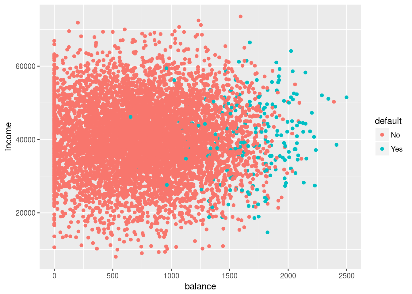

So there’s our data after removing all the student entries. Now, I’ll fit lda using the mass package.

library(MASS)

fit <- lda(default ~ balance+income, data=dataset)
fit

## Call:
## lda(default ~ balance + income, data = dataset)
## 
## Prior probabilities of groups:
##         No        Yes 
## 0.97080499 0.02919501 
## 
## Group means:
##       balance   income
## No   744.5044 39993.52
## Yes 1678.4295 40625.05
## 
## Coefficients of linear discriminants:
##                  LD1
## balance 2.258357e-03
## income  2.725668e-06

The prior probabilities and coefficients are to do with the fitting of the discriminant function, we’ll ignore those here but if you’re interested in the underlying maths have a look at Chapter 5 in Elements of Statistical Learning

The details to note is that the people will higher balances are the ones who are predicted to default. There’s also the question how good the model is, to do this we can look at various diagnostics.

Training error

The first diagnostic we’ll look at is something called the training error, it’s how often the model is correct if you we’re to predict the same \(y_i\)’s using the \(x_i\) corresponding to it and the model we fit.

#obtain predictions 
train.preds <- predict(fit)
#find % which are correct
train.err <- mean(train.preds$class==dataset$default)
train.err

## [1] 0.9757653

This is ridiculously high for a model, but this percentage is often misleading, for example let’s try another model as such, we just say nobody defaults.

#Initialize
dummypred <- dataset$default
#Change all to No, first entry is no so use that
dummypred <- dummypred[1]
mean(dummypred==dataset$default)

## [1] 0.970805

Yeah so initially we got just slightly higher than an extremely stupid model, sounds bad right? So we’ll look at why that 0.5% increase is important.

Cross Tabulation

A better way to analyse classification results is known as a cross tabulation. You simply look at a table like so:

## Num of training errors 
n-sum(train.preds$class==dataset$default)

## [1] 171

#Make crosstab
table(train.preds$class,dataset$default)

##      
##         No  Yes
##   No  6838  159
##   Yes   12   47

This is far more interesting than the number, it shows us the breakdown of the training error so the horizontal axis is the predictions and vertical is the true labels. 12 of our 171 errors occurred by saying No to people who actually do default, the other 159 were saying yes about people who actually don’t default. Now we’ll look at why LDA can be more useful.

A benefit of LDA

LDA is a statistical model, if the assumptions turn out to be true (they almost never are) we get a pretty good estimate of \(P(Y=k|X=x)\). Even when they’re not true the estimate is pretty close, so here we’ll look at the probabilities for the miss classified observations.

#index of misclassifications
miscl <-train.preds$class!=dataset$default
misclYes <- miscl & dataset$default=="Yes"
misclNo  <- miscl & dataset$default=="No"
colarray <-rep("Correct,Yes",n)
colarray[dataset$default=="No"] <- "Correct, No"
colarray[misclYes]<- "Wrong, Yes"
colarray[misclNo]<- "Wrong, No"
colarray <- as.factor(colarray)
ggplot()+geom_boxplot(aes(y=as.numeric(train.preds$posterior[,1]),x=colarray))+ylab("Probability of No")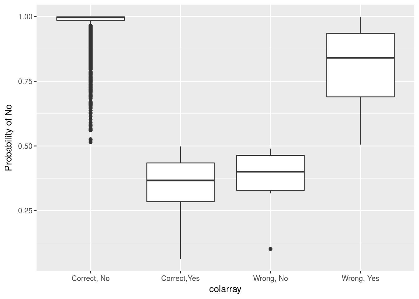

There’s a few things to note from this:

Correct, No: this is quite good as most of the probabilities are up around 1 meaning we’re usually fairly certain that they won’t default with few cases down lower past 0.9.
Correct, Yes: most of these probabilities lie in the [0.7,0.6] range of predicting they will default. Meaning we can rarely strongly state that the person will default.
Wrong, No: when the prediction was wrong but the true answer was no. This is extremely good as nearly all points are in the [0.35,0.45] range of being No which means our model doesn’t do too badly here.
Wrong, Yes: Most of these have quite a low probability of being Yes which is disappointing as it shows our model does poorly.

If you went for a rule of something like “if the model is more than 10% uncertain, carry out further checks” may be a good decision. However even the observations which we predicted correctly (Correct, yes, no) have quite a large amount of uncertainty for some observations so this may result in unneccessary work which may be avoided by using a different model or dataset.

An analysis like this would be impossible with k-nearest neighbours therefore motivating our choice. Statistical models usually give other insights which can then be useful for assessing risk or making decisions.

Conclusion

We looked at some basics of classification and how to fit a statistical classifier. Then looked at the training error rate and how it can be misleading by comparing to a dummy classifier. The cross tabulation can often be a good tool to check where the model does poorly and can be used for any classifier.

The final analysis on the probabilities is quite a desirable property of a model and is often impossible to do with other types of models. It gives you uncertainties about your predictions.

In the future, I’ll do a brief blog post on model validation and comparison which will move onto the topic of picking which model is best.